An agent is any identifiable individual (be it person or machine) that has things done to it and in turn does something. This emphasis on the doing is the hallmark of models where the relationships are based on thinking about how things happen in the real world (operational thinking). Thus, in many respects, well-formed dynamic models all tend to encapsulate the behavior of agents. The distinction we will draw for agent base models is that the individual identified as the agent will also be named in the model.
There are two approaches to directly representing agents in Stella. The first is to use modules, so each module represents an agent and can be so named. The second is to use arrays, so that each array element represents an agent. We will discuss these approaches in turn, using the same example so that they can easily be compared.
The Beer Game is a board game most commonly played with multiple teams of four or eight players. Each team represents a supply chain for the production and sale of beer, with four designated positions: retailer, wholesaler, distributor, and producer. For more information on the beer game see http://web.mit.edu/jsterman/www/SDG/beergame.html.
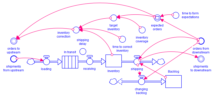
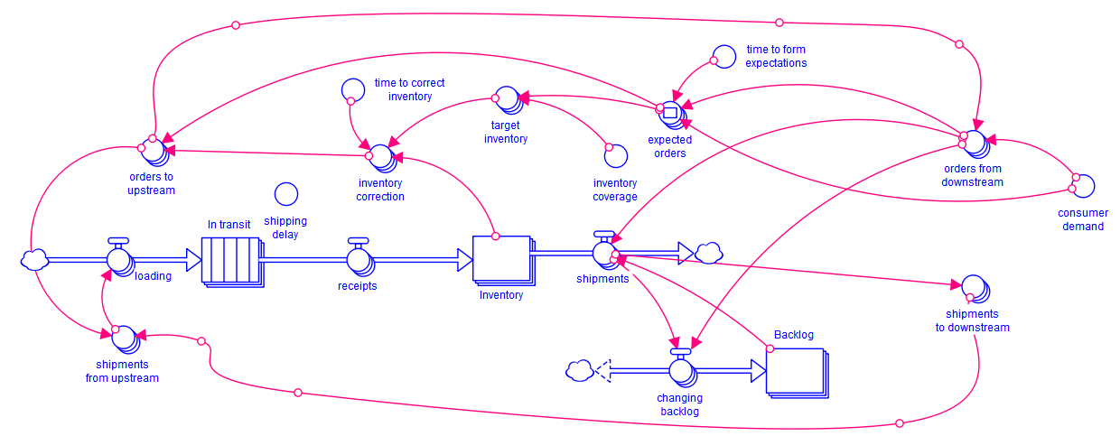
We will treat each position in the game as an agent, even through there might be one or two people playing a position depending on how the game is set up. The logic for receiving and responding to orders from downstream (toward the final customer) by making requests of the agents upstream (toward the producer). The following structure captures this decision making and the associated flows of material:
In dealing with the downstream agent (the final consumer for the retailer as an example) this agents receives order and ships. When things are working correctly those two values are the same, but if there is not enough inventory to fill orders, it may be necessary to record a backlog. The loading and receiving functions are included within the agent so that we can use the above structure for all agents without distinguishing the retailer. This could be dealt with in other ways. This model is available in the isee Exchange as StationAgent01.
Now that we have defined the stations, we need to define how the stations connect to one another to see what happens when the agents interact in the game. If you look at the above model you will see that it has inputs and outputs defined to do this working with modules, but we can use the same structure as a basis for working with arrays.
We can put the modules together in sequence by using outputs from one module as inputs to another. Configuring this way we get the model:
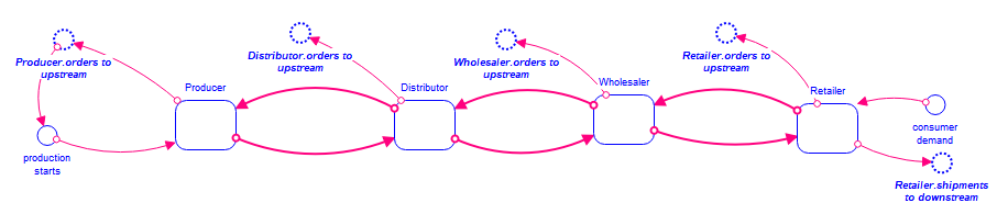
The model is constructed by putting down the modules and using the Import button on the Module Properties Tab to bring in the StationAgent01 model described above for each module. Once that is in place the inputs and outputs are connected by right clicking on the input (the variable that will use the value from another module) and assigning an output (the variable that will be used) as described in Context Menu. For example, in the Retailer module right click on shipments from upstream and assign Wholesaler.shipment to downstream using the Assign Input To menu item. We have also placed cross level ghosts for the different order placements to see how they compare to one another on a graph.
The Producer, instead of making requests of another agent simply starts production on the amount they want to order. The customer simply takes delivery of what the Retailer can ship. This model is available on the isee Exchange as DistributionGame01.
When put together this way and given a 20% step increase in consumer demand, the model produces the following behavior:
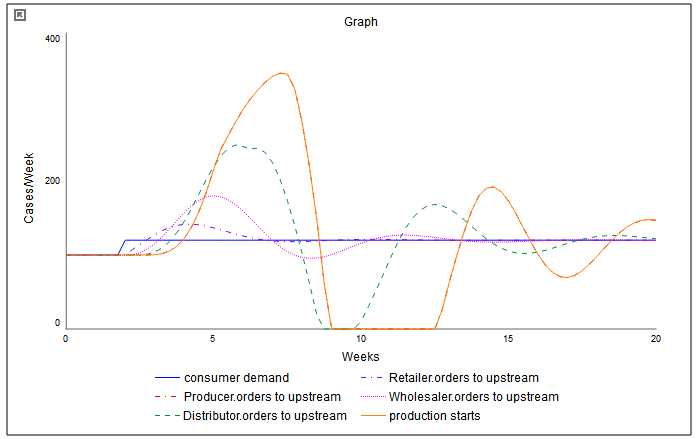
This is the classic bullwhip behavior where each successive agent in the chain has more pronounced changes in behavior. The 20% increase in final demand produces a threefold increase in production and then several weeks of not production. This is typical of the kind of amplification seen when playing the game with real players.
The station agent looks at demand and inventory to make ordering decisions, but pays no attention to what has already been ordered. While this is not far off from the way people playing the game behave, it is clearly not taking into account some pretty obvious information. We can easily add supply line correction into the station agent by tracking orders placed against receipts (something that is often, but not always, the same as the material in transit. This is done in the model StationAgent02.
With the new station agent model done, we can go to each module in the full model and replace the contents with the new model, again using the import button. The existing cross level connections will be maintained when we do this. The resulting full model looks identical; it is only the module contents that differ. The behavior becomes:
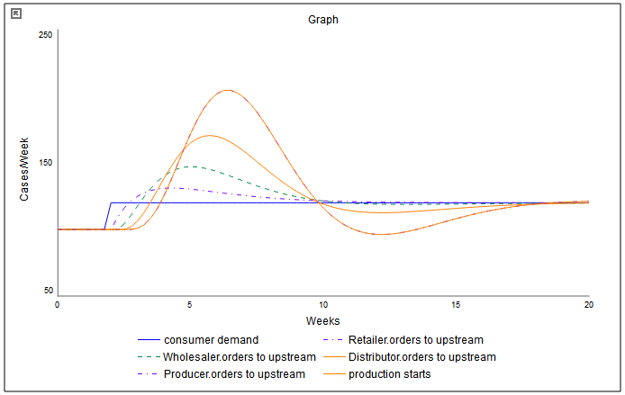
This still shows significant amplification, but is much less extreme than the original behavior.
This shows how to set up, use, and update modules to act as agents in agent based modeling. It is practical when the number of agents is relatively small, and valuable when the relationship between the agents is well expressed with connectors between modules as it is here.
We can use exactly the same station agent, and add arrays to mark the different positions:
Here the trick is just making the connections from what were marked as outputs to what were marked as inputs. This is done with the connecters, and then the equations the show how the agents interact. For example, the equation for orders from downstream becomes:
IF Position = Position.Retailer THEN consumer_demand ELSE orders_to_upstream[Position-1]
and the equation for shipments from upstream becomes:
IF Position = Position.Producer THEN orders_to_upstream[Producer] ELSE shipments_to_downstream[Position+1]
Note We also changed the equation for expected orders to use consumer demand as its initial value to avoid a simultaneous initial condition problem.
This model is available on the isee Exchange as DistributionGameArrayed. It generates exactly the same behavior as the module based model. This representation loses the station to station connectivity that the module based model clearly depicts, but at the same time offers more flexibility for changing agents by using, for example, non apply-to-all equations.
A very common thing for agents to do is to have some location at which they are active. Typically there will be a fairly large number of agents, so this type of model is best done using arrays in the current version of Stella. We make the array elements the agents, and have a variable representing the position of the agent.
For this example consider cows grazing in a field. We will represent each cow as an individual agent. Each cow grazes in a location until it looks like the grass nearby is higher, then it move to the next location. The grass grows in each location, but not as fast as the cows can eat it. We break the field up into 100 sections using a 10 x 10 grid and then look at the location of cows within that grid.
The model for this looks a little bit different from most stock and flow representations:
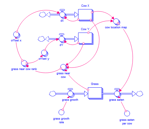
The top to stocks are arrayed by cow. The values of the stocks tell us where the cows are in the field. The stock for grass is arrayed by x and y. The movement of the cows is dependent on the height of the grass in the area around them. The equations for this are a little bit tricky, and require an additional subscript for the (up to) 9 adjacent squares. The equation for grass near cows:
Grass[Cow_X[Cow] + (Xx - 2), Cow_Y[Cow] + (Yy - 2)]
Makes use of the convention that out of range array elements will return 0 when used in this manner - effectively no grass in the squares beyond the border.
This model is available at AgentBasedGrazing. You can also see an animation of this model at Cow Simulation.
This example does not include very much beyond the x and y positions of the cows. But additional attributes and characteristics of the cows (such as whether they are well fed) could easily be added. The geographic computations are the hard part for this particular model.